Cost of Delay: How to Calculate It and Prioritize Projects

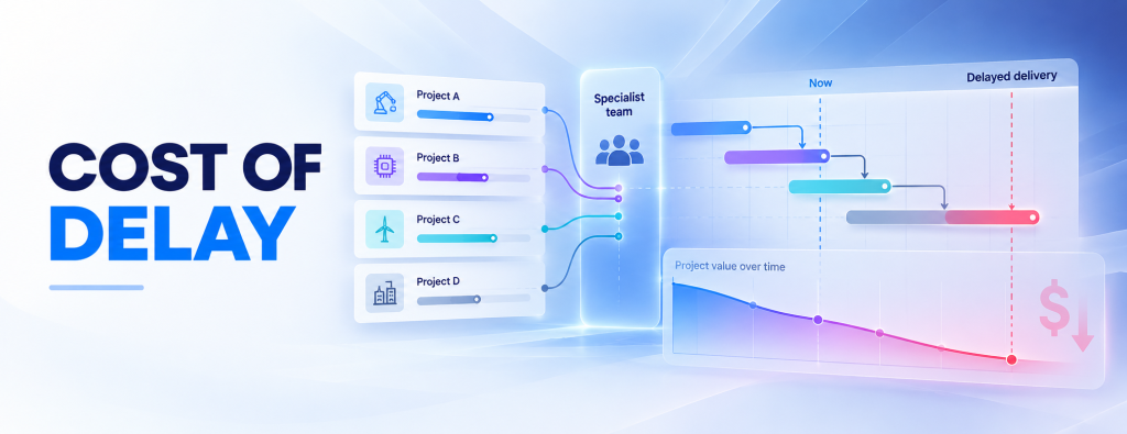
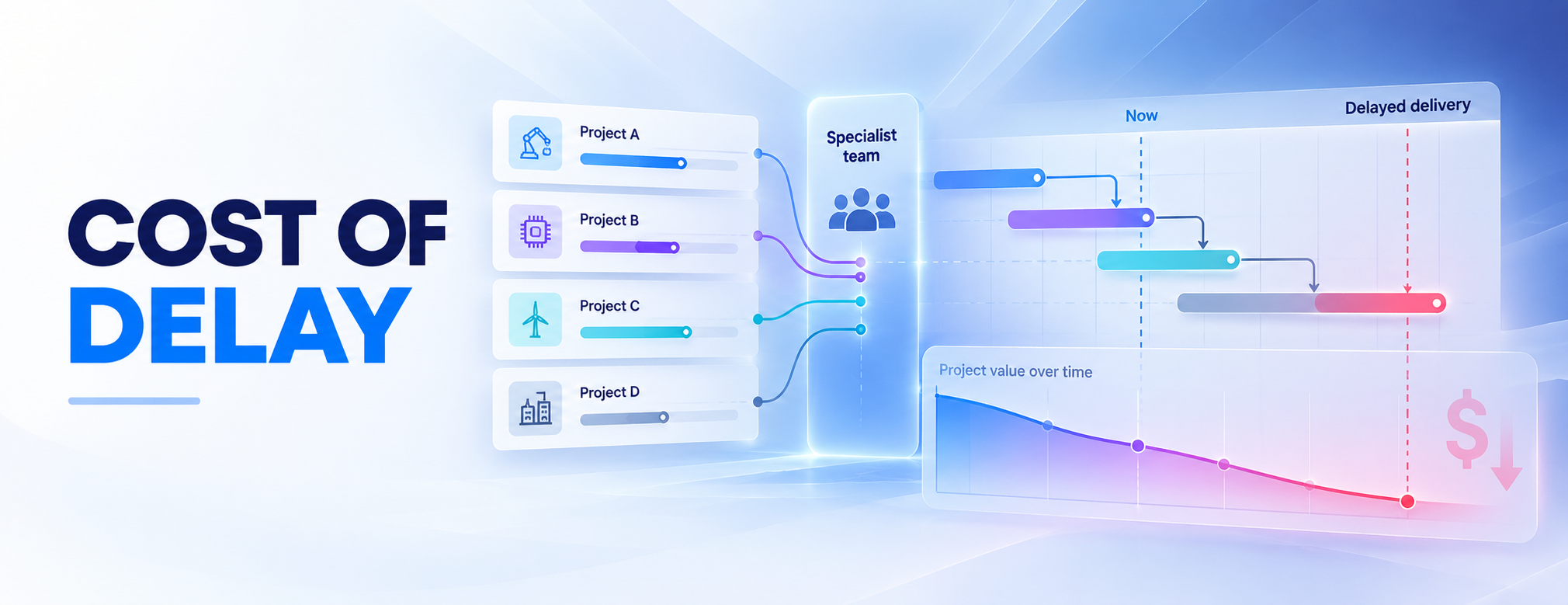
Every week a project waits for the same specialist team has a price. Cost of delay is how you put a number on it.

Short answer: Cost of delay (CoD) is the expected economic value lost by delivering an outcome later rather than sooner. It is usually expressed as a rate, such as dollars per week. If the rate is constant, the loss over a delay equals the rate multiplied by the length of the delay.

Most portfolios already rank their work by "a sense of urgency". Nobody talks about a sense of revenue, because revenue is a number. Urgency can be one too. The largest project, or the loudest request, is not always the most expensive one to postpone. This guide shows how to price the wait, compare delivery orders on one shared team, and decide whether speeding up one project is worth what it does to the others.

Key takeaways

• A CoD rate ($ per week) and a total delay cost ($) are different numbers. Keep them apart.
• Price the value you lose, not the revenue you move: contribution, savings, penalties and the time value of later cash.
• CD3, cost of delay divided by duration, orders a simple queue of ready work. It is not the best order for a whole portfolio.
• With a shared team, a week gained on one project is borrowed from another. AI capacity follows the same rule: it pays only at the bottleneck.

What is cost of delay?

Cost of delay joins value and time in one question: if this outcome arrives a week later, how much less is it worth?

Don Reinertsen made the idea central to product development economics in The Principles of Product Development Flow (2009). Joshua Arnold at Black Swan Farming later turned it into practical methods for ordering work. Cost of delay in project management works the same way: any project that releases revenue, savings or lower risk when it finishes has one.

The cost starts before the deadline, often before the work begins. A project waiting six weeks in a busy team's queue is already losing value while its status stays green.

It also explains why prioritization feels political. When nobody can price the trade-off, the loudest sponsor wins. Give the wait a price, and the argument becomes a comparison of two figures.

CoD is not a strategy on its own. Safety, legal obligations and strategic fit are limits on the decision, not values to trade against a weekly rate.

Cost of delay vs. project cost

Project cost is what it takes to do the work. CoD is what changes because the result arrives later. A $2 million program can have a low CoD, and a $200,000 fix that unblocks a customer contract a very high one.

Cost of delay rate vs. total delay cost

The rate is money per unit of time: $20,000 per week. The total is money: $60,000 for a three-week slip. In formulas and tables, keep the units apart.

The rate is also separate from lifetime value. An internal platform may enable large future revenue, but if no customer work waits on it yet, a week's slip costs little today. Its CoD is inherited from the work it blocks.

The cost of delay formula: rate vs. total loss

The basic formula multiplies a rate by a duration. Every cost of delay calculation uses one of three forms:

Formula	Use it when	Units
Total delay cost = CoD rate × delay	The weekly loss is roughly constant	$ per week × weeks = $
Total delay cost = sum of the weekly losses	The rate changes from week to week	$
Total delay cost = value if on time - value if late	Deadlines, ramp-ups, deferred payments	$, same currency and valuation date in both

An illustrative example: a product line sells $50,000 a week at a 40% contribution margin, and sales lost while you are late do not come back. The rate is $50,000 × 40% = $20,000 per week. A three-week slip costs $60,000, not $150,000. The loss is the contribution, not the revenue.

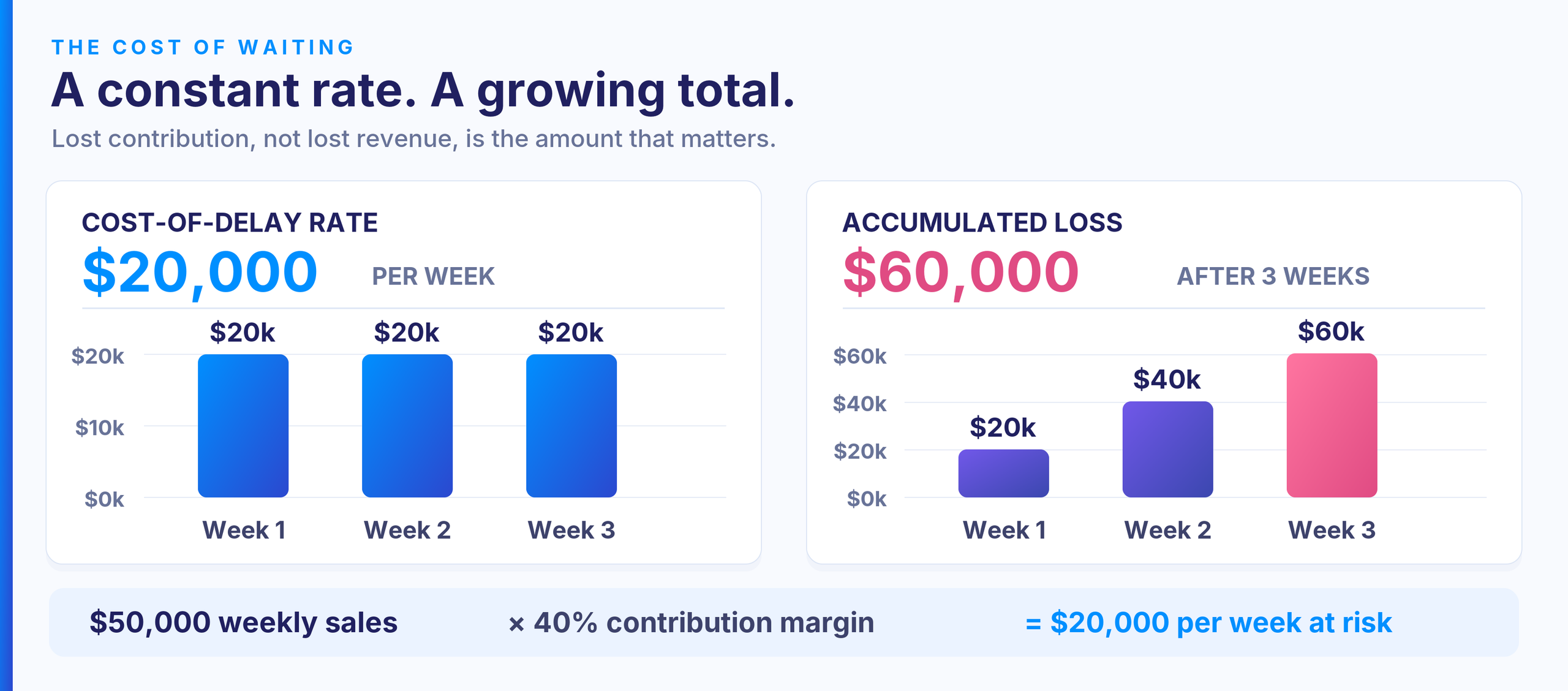
Figure 1. Constant cost-of-delay rate versus accumulated loss over three weeks. Illustrative.

When a simple formula is not enough

A constant rate breaks when a deadline triggers a penalty, when value ramps up after launch, when a market window shrinks, when risk changes over time, or when a payment is only deferred.

Deferred payments are the most overstated case. If $1,000,000 arrives one month later and nothing else changes, you have not lost $1,000,000. At a 12% effective annual rate, measured against receiving it today, the present-value loss is about $9,400: $1,000,000 - $1,000,000 / 1.12^(1/12) = $9,399.60. Name the rate and the dates. If your NPV model already includes the shift, do not add it again.

What should you include in cost of delay?

Include every economic effect that differs between the two dates, and count each one once.

Component	Evidence and owner	Counting rule
Lost contribution	Order forecast and variable costs; commercial owner with Finance	Only sales truly lost within the horizon, at contribution margin
Foregone savings	Operating cost baseline; operations owner	Only costs that would actually stop. Freed hours are capacity, not cash
Extra costs caused by the slip	Rental, support and contractor quotes; delivery owner	Only costs that differ between the dates. Never sunk spend
Bonus and penalties	Signed contract terms; commercial owner	Apply grace periods and caps. A capped penalty stops; other losses may not
Risk exposure	Risk register with stated probabilities; risk owner	The difference in expected loss. Confidence is not a probability
Timing of cash	Payment terms, invoiceable milestones; Finance	Deferred cash costs its time value, not its full amount

Give each benefit an ID, so one lost contract margin does not reappear as opportunity cost and again as a portfolio effect. Leave out a fixed team's salaries: they are paid in both scenarios. The wider model is in our guide to project financials.

Start with the numbers nobody can argue down. A contract penalty for late delivery, or a bonus for early delivery, is a date the customer has already priced. It needs no internal negotiation, and it sets a scale for valuing projects that have no contract price. For outcomes that are harder to price, treat business value in project management as a testable hypothesis.

How to calculate cost of delay in 6 steps

These six steps are a working cost of delay framework for a PMO and Finance. Each step has an owner, because a figure without an owner is not evidence.

1. Define the outcome and the dates. Name the baseline date, the later date and when the value starts. Completion is not always the start of the benefit: certification or customer acceptance can come later.

2. Estimate the incremental value from the components above. Finance confirms the basis and what is excluded.

3. Fix the units: one currency, one valuation date and one time unit for every project. Business days and calendar days are not interchangeable.

4. Model how delay changes the value: constant, a step at a deadline, or growing as a window closes. If several dependent tasks produce one outcome, count it once.

5. Check duration, capacity and readiness. Your bottleneck is a resource constraint: the specialists every project needs at the same time. The delivery owner confirms the remaining work and when that team is actually free. Use processing time, not a lead time that includes queueing. A newcomer with a higher rate is not an automatic order to stop half-done work; price the interruption first.

6. Test the uncertainty and record the decision. Use low, base and high values, find the assumption that would flip the decision, and name an owner and a review trigger.

If some of these inputs do not exist yet, that is your first finding.

Cost of delay template: a worksheet for PMO and Finance

Copy this table for each outcome you compare. The example values are illustrative and follow the product line example above.

Field	Example	Who checks what
Outcome and benefit owner	Product line launch; product line owner	Accountable for the benefit, not only delivery
Benefit start, earlier vs. later	Week 0 vs. week 3	Delivery owner: same acceptance criterion in both?
Value basis, horizon, units	Incremental contribution; fixed 12-week window; USD per week	Finance: is the value lost once the window closes?
Evidence and date checked	Signed order forecast, variable-cost estimate; [date]	Commercial and Finance
Low / base / high rate	$10,000 / $20,000 / $30,000 per week	Three sets of assumptions, not a probability
Delay cost at 3 weeks	$30,000 / $60,000 / $90,000	Constant rate assumed
Duration, capacity, dependencies, contract terms	[remaining work, team availability, prerequisites, grace period, cap]	Delivery owner: can the date really move?
Acceleration option and effect elsewhere	[change, extra spend, projects that slip]	PMO: what gets worse outside this project?
Decision and review trigger	[scenario, approver, review date]	Revisit when duration, capacity or contract terms change

Cost of delay prioritization: CD3 vs. WSJF

To decide what goes first, you need two things: what a week is worth, and how long each job keeps the bottleneck team busy. CD3 and WSJF both divide urgency by size. They measure urgency differently. For scoring models, matrices and other project prioritization methods, see our separate guide.

CD3: cost of delay divided by duration

CD3 = CoD rate / duration on the bottleneck team

Start with the highest score. Dollars per week divided by weeks gives a ranking number, not money lost per week. Black Swan Farming explains the method and its conditions in its guide to WSJF and CD3.

The logic is older than software. Goldratt's Theory of Constraints ranked factory products by the throughput they earned per hour of the scarcest machine. CD3 carries that instinct into project work: the job that earns the most per week of the scarce team goes first. In a live portfolio, where value decays and the bottleneck shifts as plans change, the measure becomes value per constrained resource hour [link to Flow Economics: add live URL or remove].

How SAFe uses relative WSJF scores

The Scaled Agile Framework estimates CoD in relative points, not money:

• Relative CoD = user-business value + time criticality + risk reduction / opportunity enablement
• WSJF (weighted shortest job first) = relative CoD / relative job size

So (8 + 5 + 3) / 2 = 8 is a score. It is not $8 and not 8% ROI. Scores only compare work estimated on one scale by one group: a 13 from one team does not mean more money than an 8 from another. See SAFe's own WSJF guidance.

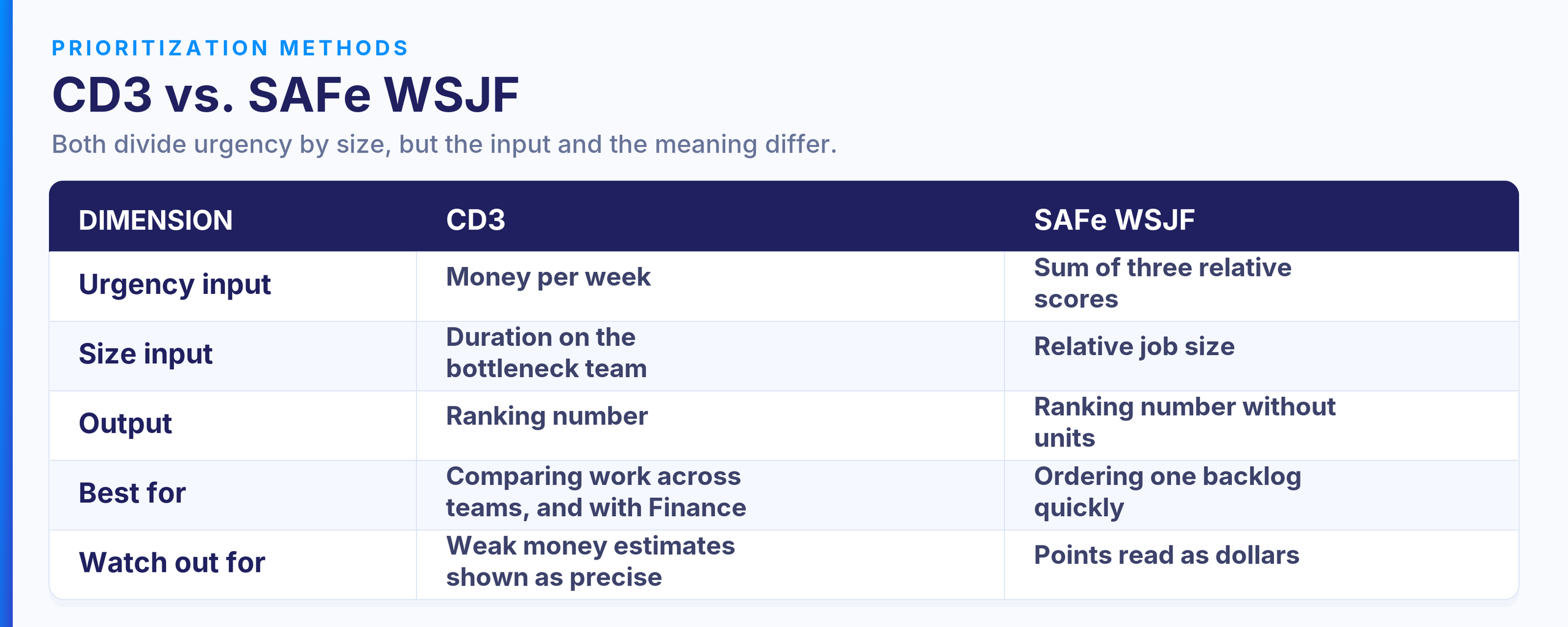
Table 1. CD3 uses monetary urgency and team duration; SAFe WSJF uses relative scores and size.

Cost of delay example: three projects, one shared team

Three projects are ready to start. All three need the same qualified team, which works on one project at a time. The figures are illustrative, not a customer case.

Project	Duration on the team (weeks)	Rate ($ per week)	CD3 score
A: equipment-control integration	6	30,000	5,000
B: production reporting automation	2	24,000	12,000
C: test-data handover improvement	1	8,000	8,000

The assumptions: all three are ready at week 0, run one after another without interruption, have no dependencies or deadlines, and deliver value from the week they finish. The rates are lost economic benefit, not revenue. Every week a project is unfinished costs its rate, so each project's loss is its rate times its completion week.

Strategy	Order	Completion week A / B / C	Loss A / B / C	Total loss
First in, first out (also highest rate first)	A → B → C	6 / 8 / 9	$180,000 / $192,000 / $72,000	$444,000
Shortest job first	C → B → A	9 / 3 / 1	$270,000 / $72,000 / $8,000	$350,000
Highest CD3 first	B → C → A	9 / 2 / 3	$270,000 / $48,000 / $24,000	$342,000

Check B → C → A week by week. In weeks 1 and 2, all three outcomes are missing: 2 × $62,000 = $124,000. In week 3, A and C are missing: $38,000. In weeks 4 to 9, only A is missing: 6 × $30,000 = $180,000. The total is $342,000.

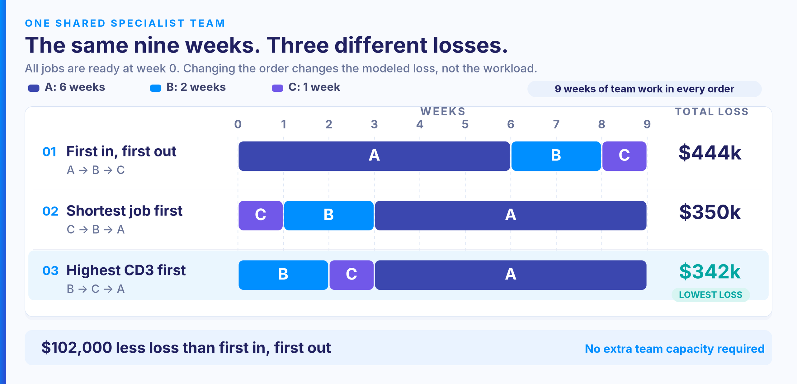
Figure 2. Three project sequences, each using the same shared team for nine weeks. Illustrative.

The team still does nine weeks of work. Only the order changes, and with it the modeled loss: $102,000 less than first in, first out. A has the highest rate, yet it goes last, because B frees the team quickly while carrying a high rate. All six possible orders were checked; B → C → A is the lowest in this model. This is a sequencing result under the stated assumptions, not a savings forecast.

Part of the loss is unavoidable: even with a team per project, the work itself takes time, worth $236,000. Waiting for the shared team adds the rest: $208,000, $114,000 and $106,000 for the three orders.

Why is the order the lever? The team's salaries are paid whichever project it works on. No scheduling choice saves money on the resource line. It moves value between projects, and the net result only shows across the portfolio.

With a fixed team, every scheduling choice moves money between projects, and cost of delay shows which way it moves.

How sensitive is the answer? B scores 12,000 ($24,000 / 2) and C scores 8,000 ($8,000 / 1). If B takes three weeks, they tie. Beyond three weeks, C should go first. So ask the delivery owner how sure they are that B takes two weeks and not three.

How time sensitivity changes cost of delay

A constant rate is only one shape. Three are common in project portfolios:

• Constant: each week of delay costs about the same, as in the example above.
• Fixed date: little or no loss until a date, then a step, such as a penalty, a missed trade show or a lost tender.
• Shrinking window: each week costs more than the last, because early sales are not recovered.

These illustrate how the model behaves; they are not an official classification. Black Swan Farming describes several urgency profiles in more depth.

Fixed-date work is where planning most often fails. A zero penalty today does not mean the start can wait. The latest safe start is the deadline minus the remaining duration, counted on the bottleneck team's real calendar. Miss it, and the penalty is certain long before the deadline.

For a shrinking window, add up the weekly losses instead of multiplying one average rate. Flow Economics shows why two projects losing the same month do not lose the same money, and when a straight-line rate puts projects in the wrong order.

From project cost of delay to critical path drag cost

CoD prices a project's lateness. Drag cost finds the activity that causes it. Both ideas come from Stephen Devaux: critical path drag is how much one activity extends the project's finish date, and drag cost is that extension times the project's CoD rate.

Drag is not the activity's duration. Two parallel paths lead to one final milestone. Path 1 is Task A (10 working days), then Task B (8): 18 days. Path 2 is Task C: 15 days. Remove Task B entirely, and the project takes 15 days, not 10, because Path 2 becomes the longest. So B's drag is 3 days, not 8.

At $10,000 per working day, B's maximum drag cost in this model is $30,000. If cutting B by five days costs $12,000 and harms nothing else, the net modeled benefit is $18,000. Whether more people would actually shorten B is a separate assumption.

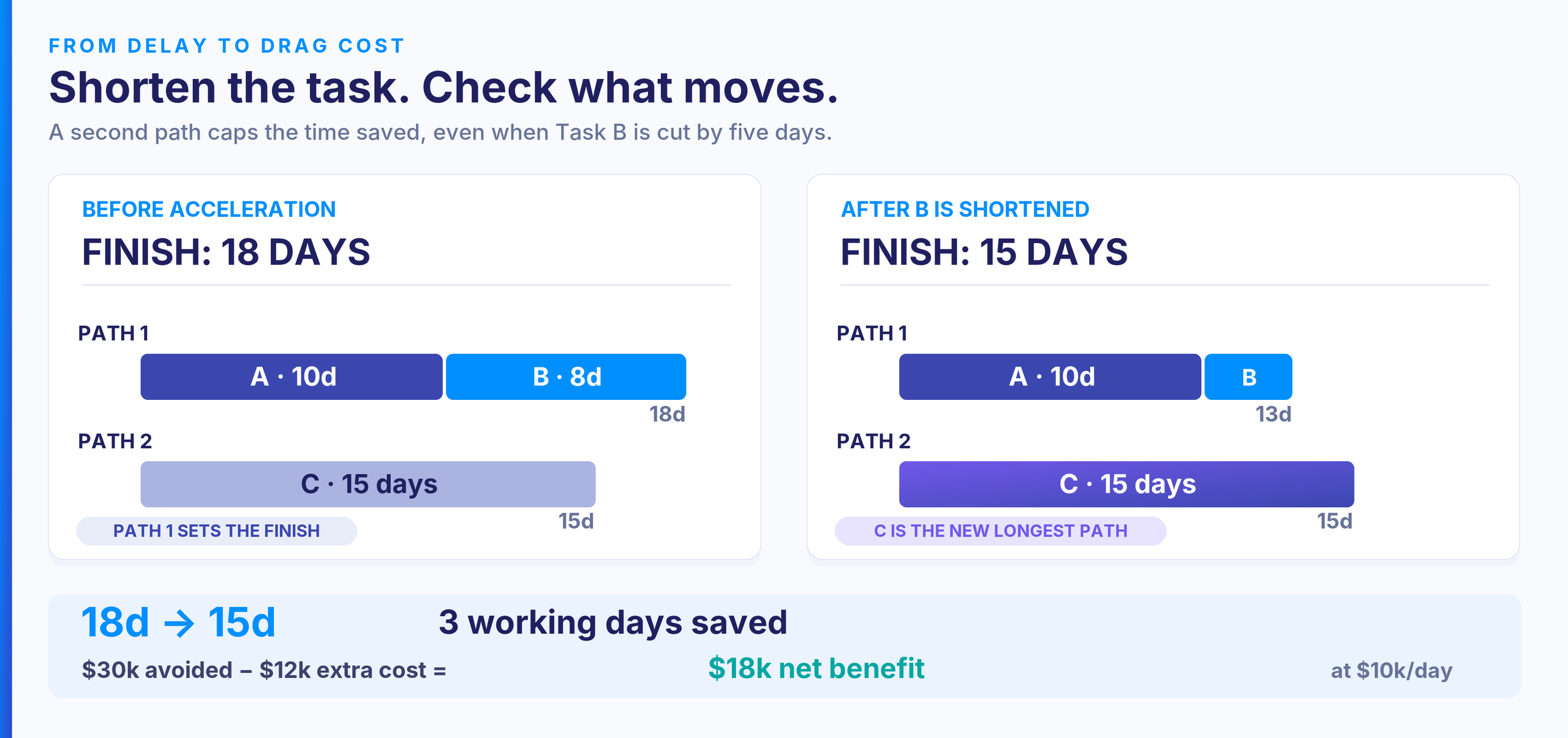
Figure 3. Parallel paths show why shortening Task B by five days saves only three days of project time. Illustrative.

Two cautions. Drag costs do not add up across tasks: shorten one path, and the next move pays less, so recalculate after every change. And the finish is not the only date that carries money. A stage payment or a certification has its own longest path, and an activity far from the critical path can still be the one delaying a payment. Price it against that milestone, not the end date.

Devaux explains the method in his article on our blog. For a shorter introduction, Flow Economics covers drag cost as the hidden price of project delay.

When is faster delivery worth paying for?

Acceleration pays only when the delay it avoids is worth more than it costs, including what it costs other projects.

Net gain = avoided delay loss - acceleration cost - loss caused elsewhere

On one project, a day of acceleration is created. Across a portfolio that shares people, it is borrowed. Move a specialist from project B to project A, and A finishes three days earlier at $10,000 a day: $30,000 avoided. But B slips two days at $12,000 a day: $24,000 lost. Add $8,000 in transition costs, and the net is $30,000 - $24,000 - $8,000 = -$2,000. The local win is a portfolio loss. The most this move is worth paying is $6,000.

Scope works the same way. An optional feature adds $20,000 of lifetime contribution, costs $15,000 to build and delays the launch by two weeks in a window worth $30,000 a week. The net is $20,000 - $15,000 - $60,000 = -$55,000. Ship it in a later increment, unless it is mandatory. None of this justifies cutting safety, quality, compliance or required testing.

How to use cost of delay to prioritize AI workflows

Choosing AI workflows is a cost of delay problem, not an automation backlog. The question is not which workflow is easiest to automate. It is which wait costs the most while it lasts.

Most teams pick AI use cases by hours saved. That is how organizations end up with a familiar result: everyone is faster, and nothing finishes sooner. An hour saved where nobody is waiting moves no delivery date. An hour saved at the bottleneck moves every project queued behind it.

Three tests decide whether a workflow is worth giving to an AI resource:

1. Is delivery waiting on it? The work sits in the queue of a scarce specialist team, an approval or a knowledge holder that other work depends on.

2. Does the wait cost real money? The projects behind it carry a rate you can name.

3. Can an agent do the work to a standard a person can check and sign off?

Most candidates fail the first test. Only work at the bottleneck passes the first two.

Take two candidates and the three-project example above. The figures are illustrative.

Candidate workflow	Easy to automate?	Time saved	Delivery dates moved	Delay cost avoided
Drafting weekly status reports for 30 project managers	Yes	About 40 hours a week, spread thinly	None	$0
Preparing test data for project B on the shared team	Harder: needs data access and a reviewer	One week of the team's time	B, C and A each finish one week sooner	$62,000

The first saves more hours. The second saves more money. One week taken off B, at the front of the queue, brings B, C and A forward together: $24,000 + $8,000 + $30,000 = $62,000. The same week saved on A, at the back of the queue, is worth $30,000, because nothing waits behind A. The status-report hours are real capacity, but they turn into money only if spending falls or the time goes to the bottleneck. The easiest workflow to automate is rarely the best one to fund.

Two corrections keep the number honest. Subtract what the agent costs to build and run. And if the bottleneck team has to review the agent's output, count that time: a review that takes back half the week saved takes back half the value.

Then rank AI candidates the way you rank projects: by the delay cost they remove per week of bottleneck time they free. Plan the AI resource like any other, with capacity, a rate, dates and a person who signs off its output. Judge it on the dates it moved, not on how busy it was.

When cost of delay prioritization can mislead you

A cost of delay analysis is only as good as its inputs. These are the common failures:

• Revenue used instead of contribution.
• A contractual penalty treated as the whole CoD.
• The same benefit counted twice.
• Relative scores presented as money.
• Deadlines and dependencies ignored.
• One precise figure where only a range can be defended.
• Rates estimated once and never updated.
• Work ranked first that is not ready to start.
• Money already spent setting the priority, although it is gone in every scenario.
• CD3 treated as the best order for a portfolio with several skills, dependencies and deadlines.

CD3 gives the best order only in a simple model: one team, independent jobs that are all ready, constant rates. Real portfolios add skill groups, precedence, release dates and shared outcomes. Those need a schedule that respects capacity and a comparison of scenarios, as does portfolio prioritization in general. If the data is too weak for money, show a range and collect evidence. Do not turn points into dollars.

A deadline can reverse the CD3 order

Keep the three-project example, but add one contract term: project A carries a one-time penalty of $60,000 if it finishes after the end of week 8.

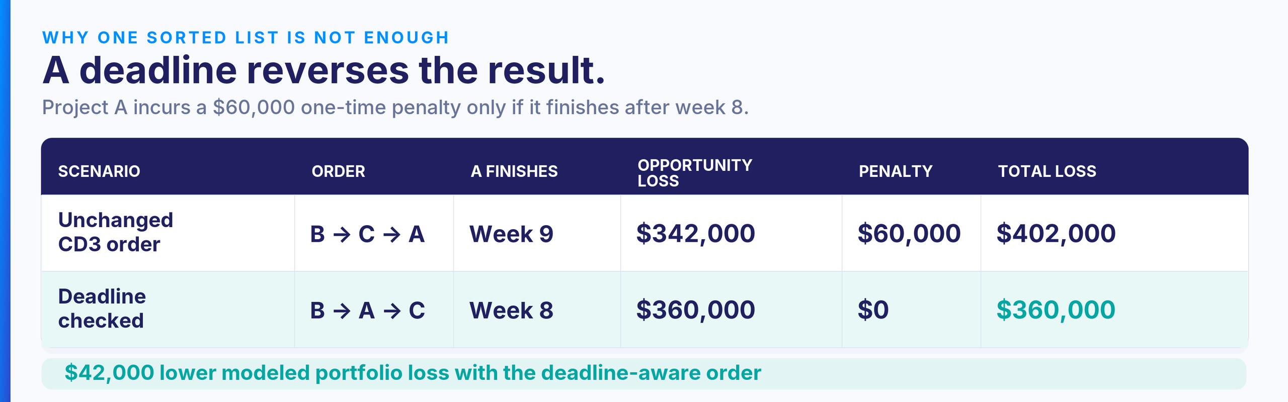
Table 2. A week-eight deadline and $60,000 penalty change the lowest-loss sequence. Illustrative.

B → A → C now wins by $42,000, and it is the lowest of all six orders. The deadline broke the constant-rate assumption, so the sorted list stopped being the answer. Recalculate whenever a date, a dependency or a contract term changes.

How Epicflow supports cost-of-delay decisions

A CoD estimate says what time is worth. It does not say whether a date is achievable, or what moving it does to the projects that share the same people. That takes a forecast of the whole portfolio.

1. Find the bottleneck. Epicflow forecasts every project from the people you actually have and shows which shared team sets the pace, months before a status report turns red.

2. Put a price on every week of delay. Attach what you already know: contract value, revenue and margin, bonus and penalty terms, invoiceable milestones. Lost revenue, later cash and penalties then move with the forecast date, while there is time to change it. The money comes from your contracts and Finance; Epicflow does not invent it.

3. Test the move first. In What-If Analysis, re-sequence, pause what can wait, move people, hire or add AI capacity, and see the new dates and cash flow for every project. Cash flow here is a schedule-derived forecast of invoiceable value, not a bank balance. Nothing live changes until you decide. An AI resource is planned like a person, with capacity, a rate and dates, whether it runs on your own agent platform or on EpicStaff, which is included with Epicflow.

4. Check whether finishing is still worth it. RRI, Epicflow's implementation of Stephen Devaux's DIPP, compares the value still to come with the cost to complete, as a multiple. See how to manage projects as investments.

Start with your own plan

Our AI searches millions of combinations for the portfolio plan that delivers the most of what you value, and today we deliver it as PMO as a Service. Send us your project list. We build a model of your own portfolio and show you, in one session, the team that holds it back, two or three ways to change the plan, and what each does to dates and money.

Test your portfolio scenario

Frequently Asked Questions

References

• Arnold, J. Cost of Delay; Four Steps to Quantifying Cost of Delay; WSJF: Weighted Shortest Job First; Urgency Profiles. Black Swan Farming. https://blackswanfarming.com/
• Devaux, S. A. (2014). Managing projects as investments: Earned value to business value. CRC Press.
• Project Management Institute. What is the economic cost of delay for software delivery? Disciplined Agile. https://www.pmi.org/disciplined-agile/what-is-the-economic-cost-of-delay-for-software-delivery
• Reinertsen, D. G. (2009). The principles of product development flow: Second generation lean product development. Celeritas Publishing.
• Scaled Agile, Inc. Weighted Shortest Job First (WSJF). SAFe Framework. https://framework.scaledagile.com/wsjf/