Epicflow – Schedule Variance: Why a Green Schedule Can Still Hide Financial Risk

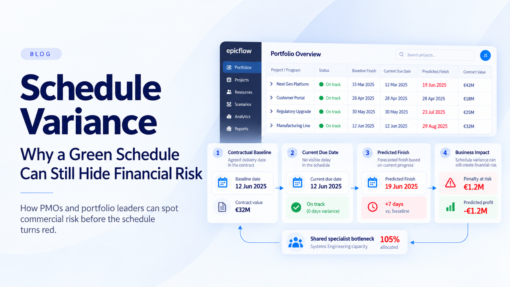
Schedule variance is a specific project management metric that quantifies project progress by subtracting planned value (PV) from earned value (EV) at a reporting cutoff date. If you get a negative result, it shows that completed work is behind project schedule. However, a reassuring earned-value status or an unchanged due date can coexist with an adverse predicted finish when shared resource constraints affect remaining tasks.

This article explains how to calculate and interpret schedule variance, then demonstrates how to separate historical reporting from capacity-aware delivery forecasts and contractual risk thresholds.

What Is Schedule Variance?

Schedule variance is an earned value management metric that compares the budgeted value of completed work with the budgeted value of work planned by a reporting date: SV = EV - PV. A positive result means progress is ahead of plan, zero means it matches plan, and a negative result means it is behind.

However, this metric alone measures historical baseline status up to the cutoff date and does not establish a project's actual or predicted finish date.

The Schedule Variance Formula: How to Calculate Schedule Variance

To understand the formula for schedule variance, we need to explain the main metrics for this calculation.

Earned value and planned value

The schedule variance formula relies on two earned value management (EVM) inputs measured at the exact same reporting cutoff date: earned value (EV) and planned value (PV).

Earned value represents the budgeted value of work actually completed by the reporting cutoff date.
Planned value represents the budgeted value of work scheduled to be completed by that same point in time.

Neither variable should ever be substituted with actual costs (AC) or commercial revenue figures.

How to calculate schedule variance

Calculating schedule variance follows a straightforward four-step sequence:

Select a specific reporting cutoff date.
Obtain comparable EV and PV values for the defined scope.
Subtract planned value from earned value (SV = EV - PV).
Interpret the resulting mathematical sign.

Both inputs must use the same budget basis, project scope, and unit of measurement. While monetary currency is common, EVM can also express inputs in budgeted labor hours, which represent effort units, not elapsed calendar days. Always compare cumulative EV against cumulative PV, but don’t mix cumulative progress with a single-period planned figure.

Note: Schedule variance percentage can be expressed as follows SV% = (EV - PV)/PV * 100, which measures the progress gap as a percentage of planned value, not percentage lateness in time.

Interpreting Schedule Variance Results (With Example)

Consider a project task evaluated at a single reporting cutoff date where planned value (PV) is $100,000 and earned value (EV) is $80,000 of completed budgeted work.

If you use schedule variance formula:

SV = EV - PV = $80,000 - $100,000 = -$20,000

The negative schedule variance result shows that the budgeted value earned is $20,000 below the planned baseline at this cutoff date. The table below illustrates alternative reporting-date outcomes for this scope:

Scenario	PV	EV	SV	SPI	Meaning
Negative	$100,000	$80,000	−$20,000	0.80	Project behind schedule and the earned-value plan
Zero	$100,000	$100,000	$0	1.00	Matches the earned-value plan
Positive	$100,000	$110,000	+$10,000	1.10	Project ahead schedule and earned-value plan

Note: These are alternative reporting-date outcomes. They do not represent sequential stages of one project's schedule.

Interpreting the gap

An SV of -$20,000 means the team has accomplished $20,000 worth of budgeted work less than scheduled by the reporting date. This figure measures budgeted progress value and should never be interpreted as a $20,000 penalty, $20,000 in lost revenue, or a 20-day delivery delay. While this earned-value status identifies past performance against the plan, it leaves crucial remaining-work sequencing and resource constraints unanswered.

Schedule Variance (SV) vs. Schedule Performance Index (SPI)

Absolute progress gap versus relative progress

Schedule variance measures the absolute dollar or effort gap in earned progress.
Schedule performance index (SPI) measures progress efficiency as a normalized ratio. The SPI formula looks like: (SPI = EV/PV).

The ratio makes relative status easier to compare across differently sized projects within a portfolio. Though it does not make their underlying deadlines or contractual exposure identical.

Dimension	Schedule variance (SV)	Schedule performance index (SPI)
Formula	EV - PV	EV/PV
Form	Absolute difference in input budget units	Unitless ratio
Favorable / On plan / Adverse	Positive / zero / negative	Above 1 / equal to 1 / below 1
Example result	-$20,000	0.80
Best use	Understand magnitude of progress gap	Compare progress relative to planned value
Shared limitation	Does not identify a feasible finish date by itself	Does not identify a feasible finish date by itself

Using EV = $80,000 and PV = $100,000, project schedule variance equals -$20,000 while SPI equals 0.80. This SPI of 0.80 means the project earned 80% of its planned budgeted progress by that cutoff, not that the total project is 80% complete or delivery will be 20% late.

Technical note: If PV = 0 at a reporting date, SPI is mathematically undefined (not applicable); do not substitute zero or 1.00. Neither metric reveals dynamic, resource-constrained finish dates on its own.

What Schedule Variance Can - and Cannot - Tell You?

Useful evidence of progress, not a complete diagnosis

Schedule variance in project management offers clear historical evidence of progress up to the reporting date, prompting early attention when actual baseline progress lags behind plan. However, the schedule variance formula alone does not describe how remaining work will be sequenced against shared resources across a portfolio.

A core requirement for reliable schedule variance reporting is data synchronization: managers must verify that EV, PV, and progress data all reflect the exact same cutoff date. Comparing stale earned-value reports against newer operational forecasts creates data-quality distortions rather than revealing true project health.

Why a reassuring result can still conceal deadline risk

Aggregate earned-value calculations suffer from critical-path blindness. Because aggregate schedule variance sums budget-weighted progress across all tasks, accumulating favorable progress on non-critical work can mask severe delays on the specific task, dependency, or scarce specialist constraint driving project completion. A favorable total schedule variance is not proof that completion-driving work is safe.

Additionally, project schedule variance exhibits an algebraic limitation near project schedule completion. For a late project that eventually finishes its baseline scope, EV and PV both reach the total baseline budget (BAC), causing schedule variance to return to zero and SPI to reach 1.00. Returning to zero simply reflects scope completion; it does not erase past calendar lateness.

Standalone SV and SPI provide valuable historical status, but advanced EVM practice and earned-schedule methods also support formal forecasting. Predictive tools for tracking project schedule complement rather than replace earned-value reporting. To investigate what the current trajectory means for a commitment, compare the contractual baseline, the administered due date, and the resource-aware predicted finish.

Why Portfolio Schedule Risk Is Different

Separate project plans, shared specialists

Evaluating schedule health in isolation overlooks portfolio-level capacity conflicts.

Consider project A undergoing critical engineering acceptance work while project B competes for the exact same qualified specialist pool. Looking strictly at project A’s reported earned-value progress omits this external demand. While a schedule variance calculation indicates past baseline progress, it does not confirm whether the remaining task sequence can execute as planned when shared experts are overloaded elsewhere.

The resource conflict represents an operational constraint to validate through capacity planning, not a root cause proven by the earned-value metric alone.

Three dates that answer different questions

Transitioning from earned-value status to delivery forecasting requires a date-based comparison. While EVM relies on a time-phased performance measurement baseline, commercial timing relies on three distinct date objects:

Contractual baseline end date. The agreed deadline that serves as the anchor for commercial rules and penalty schemas.
Current due date. The administered project date used to reflect current official schedules. It represents only an administrative setting.
Predicted end date. The dynamic, resource-aware trajectory calculated after analyzing finite specialist capacity and remaining dependencies.

Diagnosing the date gaps

Using this date-based methodology reveals forward-looking timing gaps, not the budget progress variances. Consider an evaluation on September 10, 2026, where baseline and current due dates both sit at September 30, 2026. The initial forecast projected completion on October 4, but an updated prediction shifts delivery to October 7.

Comparing these dates against the contractual anchor exposes the trajectory:

Administered gap: Current due date - Baseline = 0 days
Predicted gap: Predicted finish - Baseline = +7 calendar days

In this case, positive numbers indicate later delivery. Investigating this +7-day gap requires connecting the project-level delay to specific phase milestones, task dependencies, and overloaded specialist groups across the portfolio.

From Schedule Variance to Financial Impact

A threshold changes the commercial meaning

Continuing the project A scenario, both the contractual baseline end date and the administered due date remain fixed at September 30, 2026. While an earlier resource forecast estimated completion on October 4, the refreshed capacity prediction projects a finish on October 7.

Under an illustrative contract agreement, a five-calendar-day grace period extends through October 5 inclusive. It allows delivery to slip up to five days past baseline without financial consequences. The earlier October 4 forecast fell within this penalty-free window. However, the new October 7 prediction crosses the grace-period boundary by two days, creating a total baseline delay gap of +7 calendar days. Crossing this line transforms simple operational delay into potential commercial exposure.

Calendar-day delay	Penalty rule	Amount on $500,000 revenue
0-5 days	0%: Within grace period	$0
6-10 days	Fixed 2% adjustment	$10,000
11+ days	5% adjustment (capped at 5%)	$25,000

Contractual adjustments do not automatically charge a fixed amount for every late day. Under this hypothetical table schema rule, delays between 6 and 10 calendar days trigger a flat 2% penalty on total contract revenue, but not a cumulative daily rate. Applied to project A's baseline revenue of $500,000, the +7-day predicted delay maps directly to the 6-10 day bracket and generates a $10,000 financial deduction.

Note: this schema represents an illustrative contractual configuration, not a default system setting.

Why actual and predicted adjustments can disagree

To evaluate commercial exposure, let's distinguishing current states and forward-looking forecasts:

Financial & date measure	Current due-date state	Latest predicted-finish state
Date evaluated	September 30, 2026	October 7, 2026
Baseline date gap	0 calendar days	+7 calendar days
Penalty deduction	$0	$10,000
Adjusted revenue	$500,000 (actual revenue)	$490,000 (predicted revenue)
Actual costs subtracted	$300,000	$300,000
Calculated profit field	$200,000 (actual profit)	$190,000 (predicted profit)

Actual Bonus/Penalty reflects the current calculation state based on the administered due date; because the due date has not been officially moved from September 30, Actual Bonus/Penalty remains $0. "Actual" indicates the system's current baseline calculation state (it is not proof of accounting settlement or recognized financial liability).

In contrast, Predicted Bonus/Penalty evaluates the predicted end date (October 7) against the baseline and schema, exposing the $10,000 potential penalty. Subtracting this $10,000 deduction from baseline revenue yields a Predicted Revenue of $490,000.

Subtracting incurred Actual Costs ($300,000) produces a Predicted Profit of $190,000, compared to the current Actual Profit of $200,000. Critically, Predicted Profit subtracts only current Actual Costs, it does not incorporate a full estimate-at-completion (EAC) forecast of remaining work costs. This financial bridge isolates schedule-linked contract exposure, alerting management to emerging risk while intervention remains possible.

How to Respond to Adverse Schedule Variance

When you face adverse project schedule variance or an emerging delay, follow a three-stage decision framework to protect project outcomes before deadlines catch up.

Step 1. Investigate

Start with verifying data quality.
Confirm that the reporting project schedule cutoff dates and forecast inputs are completely fresh.
Next, trace the progress gap directly to the completion-driving phase, milestone, or task.
Inspect shared specialist workloads, task dependencies, decision queues, and remaining effort.
Before attributing a specific commercial outcome, confirm the contractual baseline anchor and the applicable contract schema rules.

Step 2. Simulate

Reforecast feasible completion dates.
Evaluating dynamic capacity and testing management alternatives.
Then, evaluate changing project priorities, resequencing tasks, adjusting non-essential scope, or reallocating specialized staffing across the portfolio.
When testing alternatives, evaluate the impact on other projects sharing those same resources.

Do not assume that adding generic headcount resolves a specialized expert constraint or that manually editing a phase deadline restores operational feasibility.

Step 3. Act and review

Document the approved decision, assigned owner, impacted projects, core assumptions, and the next scheduled review date.
Update the live project plan and re-run the capacity-aware prediction engine to confirm the updated trajectory.
Crucially, never reset or shift the project timeline baseline end date simply to make an adverse variance disappear; a formal contract change requires a separate authorized process, not administrative manipulation.

Proposed escalation rule: Escalate for investigation whenever a credible predicted finish drifts away from the contractual anchor or approaches a commercial threshold (even if the administrative due date and Actual Bonus/Penalty remain unchanged.) This guideline represents an operational best practice, not an automated software alert.

PMOs should establish their own review tolerances and response windows. Waiting for a negative EVM status or a non-zero actual penalty is not required before investigating a predicted delay.

How Epicflow Adds a Forward-Looking View: Managing Schedule Variance Using Project Planning Software

Epicflow is a resource-aware project management software for complex multi-project planning built on the Theory of Constraints (ToC). It integrates advanced features for project management schedule variance. Even though Epicflow does not replace earned-value schedule variance calculations, it complements them with resource-aware completion forecasts, cross-project capacity context, and prediction-linked commercial exposure.

When will work actually finish under real capacity limits?

Epicflow’s Prediction engine calculates feasible completion dates based on remaining work and shared specialist availability, while Future Load graph highlights overload bottlenecks across projects before they delay delivery.

Where is the emerging delay and what is its financial state?

Pipeline acts as a configurable decision workspace. Advanced View Settings can display Manual plan dates, Constraint dates, and Possible dates on the Gantt chart. Side-by-side financial columns display project-level commercial risk:

Metric / field	Purpose in pipeline workspace
Actual Bonus/Penalty	Shows current financial adjustments based on the administered due date.
Predicted B/P	Reflects calculated financial adjustments based on the resource-aware predicted end date.
Actual Profit vs. Predicted Profit	Compares current margin (Actual Revenue - Actual Cost) against forecast margin (Predicted Revenue - Actual Cost).

Note: Pipeline financial columns remain project-level metrics; filtering to a specific phase isolates schedule dependencies on the Gantt, not phase-level financial accounting.

What options exist to protect contractual commitments?

Epicflow separates planning simulation from contract testing:

What-if simulation: Evaluates operational alternatives (testing modified priorities, task sequences, or resource reallocations without impacting live plans.)
Project impact simulator: Located in the schema editor, this targeted tool tests specific bonus/penalty deductions for selected revenue and end-date variance inputs. It is a contract-rule tester, not a portfolio optimizer or ROI engine.

Epicflow complements earned-value management and enterprise ERP systems. It brings capacity-aware predictive context to traditional progress metrics. It does not calculate native project schedule variance formula, import EVM baselines, enforce contracts automatically, or guarantee project delivery.

Final Words

Calculating schedule variance in project management is essential for tracking progress against baseline plans, but earned-value metrics alone cannot predict resource-constrained completion dates. Comparing baseline, due, and predicted finish dates against contractual schemas exposes emerging financial risk while intervention is still possible. PMO leaders should investigate capacity conflicts before administrative deadlines catch up.

See how Epicflow complements schedule-status metrics with resource-aware delivery forecasts and portfolio-level intervention options.

Frequently Asked Questions (FAQs)

What is the schedule variance formula?

To calculate schedule variance (SV), you need to subtract planned value (PV) from earned value (EV). The schedule variance formula is:
SV = EV - PV,
at a specific reporting date. Inputs must use the same budget units, such as currency or labor hours. A positive result indicates progress is ahead of plan and a negative result means it is behind.

Is a positive schedule variance good?

Positive schedule variance (SV > 0) indicates that the budgeted value of completed work (earned value) exceeds the budgeted value of scheduled work (planned value). In earned value management, this signifies that project progress is currently running ahead of the planned baseline schedule. At the same time, it doesn't mean the project is automatically successful.

What does a negative schedule variance mean?

Negative schedule variance (SV < 0) shows that earned value is less than planned value. It means that the project has achieved less budgeted progress than was originally scheduled.

What is the difference between schedule variance and schedule performance index?

Schedule variance (SV) measures the absolute difference of budget units (such as dollars or labor hours). Formula: SV = EV - PV.
Schedule performance index (SPI) measures relative progress efficiency as a normalized ratio of earned work against planned work. Schedule performance index formula: SPI = EV/PV

Why can schedule variance be misleading near project completion?

As a project finishes its scope, earned value management (EVM) metrics mathematically converge because Earned Value and Planned Value both reach the total baseline budget. This causes SV to return to zero and SPI to reach 1.00 at project end. A late finish remains late even when SV reaches zero, requiring managers to check actual finish dates and remaining work.

Schedule Variance: Why a Green Schedule Can Still Hide Financial Risk